A Bayesian Approach to Time Series Forecasting

Today we are going to implement a Bayesian linear regression in R from scratch and use it to forecast US GDP growth. This post is based on a very informative manual from the Bank of England on Applied Bayesian Econometrics. I have translated the original Matlab code into R since its open source and widely used in data analysis/science. My main goal in this post is to try and give people a better understanding of Bayesian statistics, some of it’s advantages and also some scenarios where you might want to use it.

Let’s take a moment to think about why we would we even want to use Bayesian techniques in the first place. Well, there are a couple of advantages in doing so and these are particularly attractive for time series analysis. One issue when working with time series models is over-fitting particularly when estimating models with large numbers of parameters over relatively short time periods. This is not such a problem in this particular case but certainly can be when looking at multiple variables which is quite common in economic forecasting. One solution to the over-fitting problem, is to take a Bayesian approach which allows us to impose certain priors on our variables.

To understand why this works, consider the case of a Ridge Regression (L2 penalty). This is a regularisation technique helping us to reduce over-fitting (good explanation of ridge regression) by penalising us when the parameter values get large. If we instead took a Bayesian approach to the regression problem and used a normal prior we would essentially be doing the exact same thing as a ridge regression. Here is a video going through the derivation to prove that they are the same (really good course BTW). Another big reason we often prefer to use Bayesian methods is that it allows us to incorporate uncertainty in our parameter estimates which is particularly useful when forecasting.

Bayesian Theory

Before we jump right into it, lets take a moment to discuss the basics of Bayesian theory and how it applies to regression. Ordinarily, If someone wanted to estimate a linear regression of the form:

They would start by collecting the appropriate data on each variable and form the likelihood function below. They would then try to find the B and σ² that maximises this function:

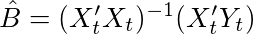
In this case, the optimal parameters can be found by taking the derivative of the log of this function and finding the values of B where the derivative equals zero. If we actually did the math, we would find the solution to be the OLS estimator below. I will not go into the derivation but here is a really nice video deriving the OLS estimates in detail. We can also think of this estimator as the covariance of X and Y divided by the variance of X.

The optimal value of the variance would be equal to

where T is the number of rows in our data set. The main difference between the classical frequentist approach and the Bayesian approach is that the parameters of the model are solely based on the information contained in the data whereas the Bayesian approach allows us to incorporate other information through the use of a prior. The table below summarises the main differences between frequentist and Bayesian approaches.

So how do we use this prior information? Well, this is when Bayes Rule comes into play. Remember the formula for Bayes rule is:

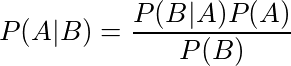
Here is a very clear explanation and example of Bayes rule being used. It demonstrates how we can combine our prior knowledge with evidence to form a posterior probability using a medical example.

Now let’s apply Bayes rule to our regression problem and see what we get. Below is the posterior distribution of our parameters. Remember, this is ultimately what we want to calculate.

Bayes Rule expressed using our model and data

We can also go a step further and describe the posterior distribution in a more succinct way.

This equation states that the posterior distribution of our parameters conditional on our data is proportional to our likelihood function (which we assume is normal) multiplied by the prior distribution of our coefficients (which is also normal). The marginal density or F(Y) in the denominator (equivalent to the P(B) in Bayes rule) is a normalising constant to ensure our distribution integrates to 1. Notice also that it doesn’t depend on our parameters so we can omit it.

In order to calculate the posterior distribution, we need to isolate the part of this posterior distribution related to each coefficient. This involves calculating marginal distributions, which in practice is often extremely difficult to do analytically. This is where a numerical method known as Gibbs sampling comes in handy. The Gibbs sampler is an example of Markov Chain Monte Carlo (MCMC) and lets us use draws from the conditional distribution to approximate the joint marginal distribution. Next up is a quick overview of how it works.

Gibbs Sampling

Imagine we have a joint distribution of N variables:

and we want to find the marginal distribution of each variable. If the form of these variables is unknown, however, it may be very difficult to calculate the necessary integrations analytically (Integration is hard!!). In cases such as these, we take the following steps to implement the Gibbs algorithm. First, we need to initialise starting values for our variables,

Next, we sample our first variable conditional on the current values of the other N-1 variables. i.e.

We then sample our second variable conditional on all the others

, repeating this until we have sampled each variable. This ends one iteration of the Gibbs sampling algorithm. As we repeat these steps a large number of times the samples from the conditional distributions converge to the joint marginal distributions. Once we have M runs of the Gibbs sampler, the mean of our retained draws can be thought of as an approximation of the mean of the posterior distribution. Below is a visualisation of the sampler in action for two variables. You can see how initially the algorithm starts sampling from points outside our distribution but starts to converge to it after a number of steps.

Source: Coursera: Bayesian Methods for Machine learning

Now that we have the theory out of the way, let’s see how it works in practice. Below is the code for implementing a linear regression using the Gibbs sampler. In particular, I will estimate an AR(2) model on year over year growth in quarterly US Gross Domestic Product (GDP). I will then use this model to forecast GDP growth using a Bayesian framework. Using this approach we can construct credible intervals around our forecasts using quantiles from the posterior density i.e. quantiles from the retained draws from our algorithm.

Model

Our model will have the following form:

We can also write this in matrix form by defining the following matrices.

B above which is just a vector of coefficients, and our matrix of data X below.

This gives us the form in equation 1 up above. As I said already our goal here is to approximate the posterior distribution of our coefficients:

and we can do this by calculating the conditional distributions within a Gibbs sampling framework. Alright, now that the theory is out of the way let’s start coding this up in R.

Code

The first thing we need to do is load in the data. I downloaded US GDP growth from the Federal Reserve of St.Louis website (FRED). I choose p=2 as the number of lags I want to use. This choice is pretty arbitrary and there are formal tests such as the AIC and BIC we can use to choose the best number of lags but I haven’t used them for this analysis. What is the old saying? Do as I say not as I do. I think this applies here. 😄

library(ggplot)

Y.df <- read.csv('USGDP.csv', header =TRUE)
names <- c('Date', 'GDP')
Y <- data.frame(Y.df[,2])

p = 2
T1 = nrow(Y)

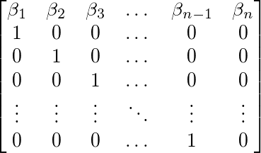
Next, we define the regression_matrix function to create our X matrix containing our p lagged GDP variable and a constant term. The function takes in three parameters, the data, the number of lags and TRUE or FALSE depending on whether we want a constant or not. I also created another helper function below this which transforms the coefficient matrix from our model into a companion form matrix. This function, ar_companion_matrix essentially transforms a coefficient matrix like the one below (Notice that the constant term is not included):

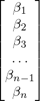
Into an n*n matrix with the coefficients along the top row and an (n-1)*(n-1) identity matrix below this. Expressing our matrix this way allows us to calculate the stability of our model later on which will be an important part of our Gibbs Sampler. I will talk about more about this later in the post when we get to the relevant code.

regression_matrix  <- function(data,p,constant){
    nrow <- as.numeric(dim(data)[1])
    nvar <- as.numeric(dim(data)[2])
    
    Y1 <- as.matrix(data, ncol = nvar)
    X <- embed(Y1, p+1)
    X <- X[,(nvar+1):ncol(X)]
    if(constant == TRUE){
        X <-cbind(rep(1,(nrow-p)),X)
    }
    Y = matrix(Y1[(p+1):nrow(Y1),])
    nvar2 = ncol(X)
    return = list(Y=Y,X=X,nvar2=nvar2,nrow=nrow) 
}

################################################################

ar_companion_matrix <- function(beta){

    #check if beta is a matrix
    if (is.matrix(beta) == FALSE){
        stop('error: beta needs to be a matrix')
    }
    # don't include constant
    k = nrow(beta) - 1
    FF <- matrix(0, nrow = k, ncol = k)
    
    #insert identity matrix
    FF[2:k, 1:(k-1)] <- diag(1, nrow = k-1, ncol = k-1)
    temp <- t(beta[2:(k+1), 1:1])

    
    #Insert coefficients along top row
    FF[1:1,1:k] <- temp
    return(FF)
}

Our next bit of code implements our regression_matrix function and extracts the matrices and number of rows from our results list. We also set up our priors for the Bayesian analysis.

results = list()
results <- regression_matrix(Y, p, TRUE)

X <- results$X
Y <- results$Y
nrow <- results$nrow
nvar <- results$nvar

# Initialise Priors
B <- c(rep(0, nvar))
B <- as.matrix(B, nrow = 1, ncol = nvar)
sigma0 <- diag(1,nvar)

T0 = 1 # prior degrees of freedom
D0 = 0.1 # prior scale (theta0)

# initial value for variance
sigma2 = 1

What we have done here is essentially set a normal prior for our Beta coefficients which have mean = 0 and variance = 1. For our mean we have priors:

And for our variance we have priors:

For the variance parameter, we have set an inverse gamma prior (conjugate prior). This is a standard distribution to use for the variance as it is only defined for positive numbers which is ideal for variance since it can only be positive.

For this example, we have arbitrarily chosen T0 = 1 and theta0= 0.1 (D0 is our code). If we wanted to test these choice of priors we could do robustness tests by changing our initial priors and seeing if it changes the posterior significantly. If we try and visualise what changing the value of theta0 does, we would see that a higher value would give us a wider distribution with our coefficient more likely to take on larger values in absolute terms, similar to having a large prior variance on our Beta.

reps = 15000
burn = 4000
horizon = 14
out = matrix(0, nrow = reps, ncol = nvar + 1)
colnames(out) <- c(‘constant’, ‘beta1’,’beta2', ‘sigma’)
out1 <- matrix(0, nrow = reps, ncol = horizon)

Above we set our forecast horizon and initialise some matrices to store our results. We create a matrix called out which will store all of our draws. It will need to have rows equal to the number of draws of our sampler, which in this case is equal to 15,000. We also need to create a matrix that will store the results of our forecasts. Since we are calculating our forecasts by iterating an equation of the form:

We will need our last two observable periods to calculate the forecast. This means our second matrix out1 will have columns equal to the number of forecast periods plus the number of lags, 14 in this case.

Implementation of Gibbs Sampling

OK, so what follows is a big complicated looking piece of code but I will go through it step by step and hopefully, it will be clearer afterwards.

gibbs_sampler <- function(X,Y,B0,sigma0,sigma2,theta0,D0,reps,out,out1){

# Main Loop
for(i in 1:reps){

    if (i %% 1000 == 0){
    print(sprintf("Interation: %d", i))
        }

    # Conditional Posterior Mean and Variance
    M = solve(solve(sigma0) + as.numeric(1/sigma2) * t(X) %*% X) %*%
        (solve(sigma0) %*% B0 + as.numeric(1/sigma2) * t(X) %*% Y)
    
    V = solve(solve(sigma0) + as.numeric(1/sigma2) * t(X) %*% X)
    
    chck = -1
    while(chck < 0){   # check for stability
        
        B <- M + t(rnorm(p+1) %*% chol(V))
        
        # Check : not stationary for 3 lags
        b = ar_companion_matrix(B)
        ee <- max(sapply(eigen(b)$values,abs))
        if( ee<=1){
            chck=1
        }
    }

    # compute residuals
    resids <- Y - X%*%B
    T2 = T0 + T1
    D1 = D0 + t(resids) %*% resids
    
 
    out[i,] <- t(matrix(c(t(B),sigma2)))
    
    
    #draw from Inverse Gamma
    z0 = rnorm(T1,1)
    z0z0 = t(z0) %*% z0
    sigma2 = D1/z0z0
    
    
    out[i,] <- t(matrix(c(t(B),sigma2)))
    
    # compute 2 year forecasts
    yhat = rep(0,horizon)
    end = as.numeric(length(Y))
    yhat[1:2] = Y[(end-1):end,]
    cfactor = sqrt(sigma2)
    X_mat = c(1,rep(0,p))

    for(m in (p+1):horizon){
            for (lag in 1:p){
            #create X matrix with p lags
                X_mat[(lag+1)] = yhat[m-lag]
             }
            #Use X matrix to forecast yhat
            yhat[m] = X_mat %*% B + rnorm(1) * cfactor
     }

    out1[i,] <- yhat

} # end of Gibbs Sampler
    
 return = list(out,out1)

    } 

results1 <- gibbs_sampler(X,Y,B0,sigma0,sigma2,T0,D0,reps,out,out1)

# burn first 4000
coef <- results1[[1]][(burn+1):reps,]
forecasts <- results1[[2]][(burn+1):reps,]

First of all, we need the following arguments for our function. Our initial variable, in this case, GDP Growth(Y). Our X matrix, which is just Y lagged by 2 periods with a column of ones appended. We also need all of our priors that we defined earlier, the number of times to iterate our algorithm (reps) and finally, our 2 output matrices.

The main loop is what we need to pay the most attention to here. This is where all the main computations take place. The first two equations M and V describe the posterior mean and variance of the normal distribution conditional on B and σ². I won’t derive these here, but if you are interested they are available in Time Series Analysis by Hamilton (1994) or in Bishop Pattern Recognition and Machine Learning Chapter 3 (Albeit with slightly different notation). To be explicit, the mean of our posterior parameter Beta is defined as:

and the variance of our posterior parameter Beta is defined as:

If we play around a bit with the second term in M, we can substitute in our maximum likelihood estimator for Y_t. Doing so gives us

Essentially this equation says that M is just a weighted average of our prior mean and our maximum likelihood estimator for Beta. I think intuitively this makes quite a lot of sense since we are trying to combine our prior information as well as the evidence from our data. Let’s consider our prior variance for a moment to try and improve our interpretation of this equation. If we assigned a small prior variance (sigma0), essentially we are confident in our choice of prior and think that our posterior will be close to it. In this case the distribution will be quite tight. Conversely, the opposite is true if we set a high variance on our Beta parameter. In this scenario the Beta OLS parameter will be more heavily weighted.

We are not done yet though. We still need to get a random draw from the correct distribution but we can do this using a simple trick. To get a random variable from a Normal distribution with mean M and variance V we can sample a vector from a standard normal distribution and transform it using the equation below.

Draw of B from conditional posterior distribution

Essentially we add our conditional posterior mean and scale by the square root of our posterior variance (standard deviation). This gives us our sample B from our conditional posterior distribution. The next bit of code also has a check to make sure the coefficient matrix is stable i.e. our variable is stationary ensuring our model is dynamically stable. By recasting our AR(2) as an AR(1) (companion form), we can check if the absolute values of the eigenvalues are less than 1 (only need to check the largest eigenvalue is <|1|). If they are, then that means our model is dynamically stable. If anyone wants to go into this in more detail I recommend chapter 17 of Fundamental Methods of Mathematical Economics or just read this blog post for a quick primer.

Now that we have our draw of B, we draw sigma from the Inverse Gamma distribution conditional on B. To sample a random variable from the inverse Gamma distribution with degrees of freedom

and scale

we can sample T variables from a standard normal distribution z0 ~ N(0,1) and then make the following adjustment

z is now a draw from the correct Inverse Gamma distribution.

The code below this stores our draws of the coefficients into our out matrix. We then use these draws to create our forecasts. The code essentially creates a matrix called yhat, to store our forecasts for 12 periods into the future (3 years since we are using quarterly data). Our equation for a 1 step ahead forecast can be written as

In general, we will need a matrix of size n+p where n is the number of periods we wish to forecast and p is the number of lags used in the AR. The forecast is just an AR(2) model with a random shock each period that is based on our draws of sigma. OK that is pretty much it for the Gibbs sampler code.

Now we can start looking at what the algorithm produced. The code below extracts the coefficients that we need which correspond to the columns of the coef matrix. Each row gives us the value of our parameter for each draw of the Gibbs sampler. Calculating the mean of each of these variables gives us an approximation of the posterior mean of the distribution for each coefficient. 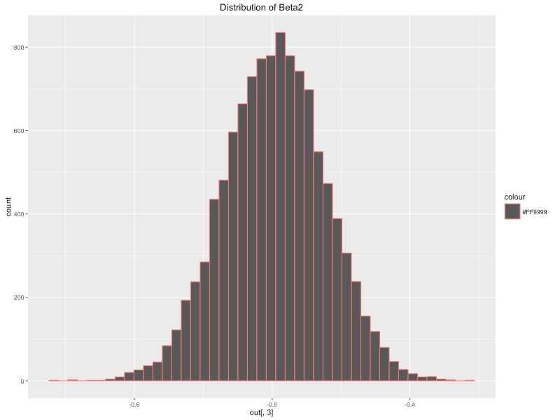This distribution can be quite useful for other statistical techniques such as hypothesis testing and is another advantage of taking a Bayesian approach to modelling. Below I have plotted the posterior distribution of the coefficients using ggplot2. We can see that they closely resemble a normal distribution which makes sense given we defined a normal prior and likelihood function. The posterior means of our parameters are as follows:

const <- mean(coef[,1])
beta1 <- mean(coef[,2])
beta2 <- mean(coef[,3])
sigma <- mean(coef[,4])

qplot(coef[,1], geom = "histogram", bins = 45, main = 'Distribution of Constant',
      colour="#FF9999")
qplot(coef[,2], geom = "histogram", bins = 45,main = 'Distribution of Beta1',
      colour="#FF9999")
qplot(coef[,3], geom = "histogram", bins = 45,main = 'Distribution of Beta2',
      colour="#FF9999")
qplot(coef[,4], geom = "histogram", bins = 45,main = 'Distribution of Sigma',
      colour="#FF9999")

The next thing we are going to do is use these parameters to plot our forecasts and construct our credible intervals around these forecasts.

Plotting our Forecasts

Below is a 3 year forecast for year over year GDP growth. Notice that using Bayesian analysis has allowed us to create a forecast with credible intervals which is very useful in highlighting the uncertainty of our forecasts. Note that this is distinct from a confidence interval and is interpreted slightly different. If we were taking a frequentist approach and ran an experiment 100 times for example, we would expect that our true parameter value would be in this range in 95 out of the 100 experiments. In contrast, the Bayesian approach is interpreted as the true parameter value being contained within this range with 95 per cent probability. This difference is subtle but pretty important.

library(matrixStats); library(ggplot2); library(reshape2)

#uantiles for all data points, makes plotting easierpost_means <- colMeans(coef)
forecasts_m <- as.matrix(colMeans(forecasts))

#Creating error bands/credible intervals around our forecasts
error_bands <- colQuantiles(forecasts,prob = c(0.16,0.84))
Y_temp = cbind(Y,Y)

error_bands <- rbind(Y_temp, error_bands[3:dim(error_bands)[1],])
all <- as.matrix(c(Y[1:(length(Y)-2)],forecasts_m))

forecasts.mat <- cbind.data.frame(error_bands[,1],all, error_bands[,2])
names(forecasts.mat) <- c('lower', 'mean', 'upper')

# create date vector for plotting
Date <- seq(as.Date('1948/07/01'), by = 'quarter', length.out = dim(forecasts.mat)[1])

data.plot <- cbind.data.frame(Date, forecasts.mat)
data_subset <- data.plot[214:292,]
data_fore <- data.plot[280:292,]

ggplot(data_subset, aes(x = Date, y = mean)) + geom_line(colour = 'blue', lwd = 1.2) + geom_ribbon(data = data_fore,
aes(ymin = lower, ymax = upper , colour = "bands", alpha = 0.2))

The code above calculates the 16 and 84 percentiles of our forecasts to use as credible intervals. We combine these columns with our forecasts and then plot a subset of the data using ggplot and geom_ribbon to plot the intervals around the forecast. The plot above looks reasonably nice but I would like to make this a bit prettier .

I found a very helpful blog post which creates fan charts very similar to the Bank of England's Inflation reports. The library I use is called fanplot and lets you plots different percentiles of our forecast distribution which looks a little nicer than the previous graph.

library(fanplot)
forecasts_mean <- as.matrix(colMeans(out2))
forecast_sd <- as.matrix(apply(out2,2,sd))
tt <- seq(2018.25, 2021, by = .25)
y0 <- 2018.25
params <- cbind(tt, forecasts_mean[-c(1,2)], forecast_sd[-c(1,2)])
p <- seq(0.10, 0.90, 0.05)

# Calculate Percentiles
k = nrow(params)
gdp <- matrix(NA, nrow = length(p), ncol = k)
for (i in 1:k) 
    gdp[, i] <- qsplitnorm(p, mode = params[i,2], 
                           sd = params[i,3])

# Plot past data
Y_ts <- ts(data_subset$mean, frequency=4, start=c(2001,1))
plot(Y_ts, type = "l", col = "tomato", lwd = 2.5, 
     xlim = c(y0 - 17, y0 + 3), ylim = c(-4, 6), 
     xaxt = "n", yaxt = "n", ylab="")

# background and fanchart
rect(y0-0.25, par("usr")[3] - 1, y0 + 3, par("usr")[4], 
     border = "gray90", col = "gray90")
fan(data = gdp, data.type = "values", probs = p, 
    start = y0, frequency = 4, 
    anchor = Y_ts[time(Y_ts) == y0-.25], 
    fan.col = colorRampPalette(c("tomato", "gray90")), 
    ln = NULL, rlab = NULL)

# BOE aesthetics
axis(2, at = -2:5, las = 2, tcl = 0.5, labels = FALSE)
axis(4, at = -2:5, las = 2, tcl = 0.5)
axis(1, at = 2000:2021, tcl = 0.5)
axis(1, at = seq(2000, 2021, 0.25), labels = FALSE, tcl = 0.2)
abline(h = 0)
abline(v = y0 + 1.75, lty = 2) #2 year line

Conclusion

Our forecast seems quite positive, with a mean prediction of annual growth at around 3 per cent until 2021. There also seems to be quite a bit of upside risk with the 95 per cent credible interval going up to nearly 5 per cent. The graph indicates that it is highly unlikely that there will be negative growth over the period which is quite interesting and judging by the expansionary economic policies in the US right now this may turn out to be correct. The confidence bands are pretty large as you can see, indicating that there is a wide distribution on the value that GDP growth could have over the forecast period. There are many other types of models we could have used instead and probably get a more accurate forecast such as Bayesian VAR’s or Dynamic Factor models which use a number of other economic variables. While potentially more accurate, these models are much more complex and a lot more difficult to code up. For the purposes of an introduction to Bayesian Regression and to get an intuitive understanding this approach an AR model is perfectly reasonable.

I think it is important to say why I have chosen to do this kind of model from scratch when there are clearly much easier and less painful ways of doing this type of forecasting. I tend to find that the absolute best way for me to learn something complex like this is to try and reproduce the algorithm from scratch. This really reinforces what I have learned theoretically and forces me to put it into an applied setting which can be extremely difficult if I haven't fully understood the topic. I also find that this approach makes things stick in my head a bit longer. In practice I probably wouldn't use this code as it is likely to break quite easily and be hard to debug (as I have already discovered) but I think this is a very effective way to learn. While this obviously takes a lot longer then just finding a package in R or Python for the task the benefit from taking the time out to go through it step by step is ultimately greater and I would recommend it to anyone trying to learn or understand how different models and algorithms work.

OK folks, that concludes this post. I hope you all enjoyed it and learned a bit about Bayesian Statistics and how we can use it in practice. If you have any questions feel free to post below or connect with me via LinkedIn.

Search This Blog

basezz.com