Mobile Ads Click-Through Rate (CTR) Prediction

f

Online Advertising, Google PPC, AdWords Campaign, Mobile Ads

Susan Li

Dec 8

In Internet marketing, click-through rate (CTR) is a metric that measures the number of clicks advertisers receive on their ads per number of impressions.

Mobile has become seamless with all channels, and mobile is the driving force with what’s driving all commerce. Mobile ads are expected to generate $1.08 billion this year, which would be a 122% jump from last year.

In this research analysis, Criteo Labs is sharing 10 days’ worth of Avazu data for us to develop models predicting ad click-through rate (CTR). Given a user and the page he (or she) is visiting. what is the probability that he (or she) will click on a given ad? The goal of this analysis is to benchmark the most accurate ML algorithms for CTR estimation. Let’s get started!

The Data

The data set can be found here.

Data fields

• id: ad identifier
• click: 0/1 for non-click/click
• hour: format is YYMMDDHH, so 14091123 means 23:00 on Sept. 11, 2014 UTC.
• C1 — anonymized categorical variable
• banner_pos
• site_id
• site_domain
• site_category
• app_id
• app_domain
• app_category
• device_id
• device_ip
• device_model
• device_type
• device_conn_type
• C14-C21 — anonymized categorical variables

EDA & Feature Engineering

The training set contains over 40 millions of records, to be able to process locally, we will randomly sample 1 million of them.

import numpy as n
import random
import pandas as pd
import gzip

n = 40428967  #total number of records in the clickstream data 
sample_size = 1000000
skip_values = sorted(random.sample(range(1,n), n-sample_size))

parse_date = lambda val : pd.datetime.strptime(val, '%y%m%d%H')

with gzip.open('train.gz') as f:
    train = pd.read_csv(f, parse_dates = ['hour'], date_parser = parse_date, dtype=types_train, skiprows = skip_values)

Figure 1

Because of the anonymization, we don’t know what each value means in each feature. In addition, most of the features are categorical and most of the categorical features have a lot of values. This makes EDA less intuitive easier to confuse, but we will try the best.

Features

We can group all the features in the data into the following categories:

• Target feature : click
• site features : site_id, site_domain, site_category
• app feature: app_id, app_domain, app_category
• device feature: device_id, device_ip, device_model, device_type, device_conn_type
• anonymized categorical features: C14-C21

import seaborn as sns
import matplotlib.pyplot as plt

sns.countplot(x='click',data=train, palette='hls')
plt.show();

Figure 2

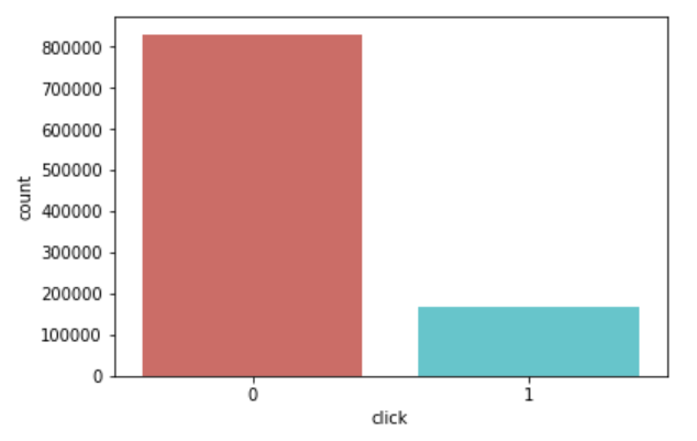
train['click'].value_counts()/len(train)

Figure 3

The overall click through rate is approx. 17%, and approx. 83% is not clicked.

train.hour.describe()

Figure 4

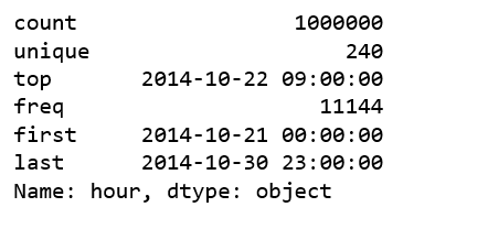
The data covers 10 days of click streams data from 2014–10–21 to 2014–10–30, that is 240 hours.

train.groupby('hour').agg({'click':'sum'}).plot(figsize=(12,6))
plt.ylabel('Number of clicks')
plt.title('Number of clicks by hour');

Figure 5

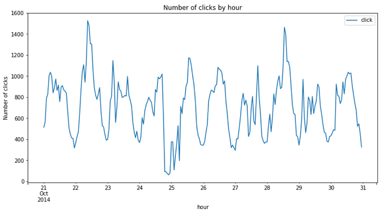
The hourly clicks pattern looks pretty similar every day. However, there were a couple of peak hours, one is sometime in the mid of the day on Oct 22, and another is sometime in the mid of the day on Oct 28. And one very low click hour is close to mid-night on Oct 24.

Feature engineering for date time features

Hour

Extract hour from date time feature.

train['hour_of_day'] = train.hour.apply(lambda x: x.hour)
train.groupby('hour_of_day').agg({'click':'sum'}).plot(figsize=(12,6))
plt.ylabel('Number of clicks')
plt.title('click trends by hour of day');

Figure 6

In general, the highest number of clicks is at hour 13 and 14 (1pm and 2pm), and the lowest number of clicks is at hour 0 (mid-night). It seems a useful feature for roughly estimation.

Let’s take impressions into consideration.

train.groupby(['hour_of_day', 'click']).size().unstack().plot(kind='bar', title="Hour of Day", figsize=(12,6))
plt.ylabel('count')
plt.title('Hourly impressions vs. clicks');

Figure 7

There is nothing shocking here.

Now that we have looked at clicks and impressions. We can calculate click-through rate (CTR). CTR is the ratio of ad clicks to impressions. It measures the rate of clicks on each ad.

Hourly CTR

import seaborn as sns

df_click = train[train['click'] == 1]
df_hour = train[['hour_of_day','click']].groupby(['hour_of_day']).count().reset_index()
df_hour = df_hour.rename(columns={'click': 'impressions'})
df_hour['clicks'] = df_click[['hour_of_day','click']].groupby(['hour_of_day']).count().reset_index()['click']
df_hour['CTR'] = df_hour['clicks']/df_hour['impressions']*100

plt.figure(figsize=(12,6))
sns.barplot(y='CTR', x='hour_of_day', data=df_hour)
plt.title('Hourly CTR');

Figure 8

One of the interesting observations here is that the highest CTR happened in the hour of mid-night, 1, 7 and 15. If you remember, around mid-night has the least number of impressions and clicks.

Day of week

train['day_of_week'] = train['hour'].apply(lambda val: val.weekday_name)
cats = ['Monday', 'Tuesday', 'Wednesday', 'Thursday', 'Friday', 'Saturday', 'Sunday']
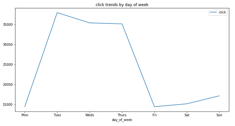
train.groupby('day_of_week').agg({'click':'sum'}).reindex(cats).plot(figsize=(12,6))
ticks = list(range(0, 7, 1)) # points on the x axis where you want the label to appear
labels = "Mon Tues Weds Thurs Fri Sat Sun".split()
plt.xticks(ticks, labels)
plt.title('click trends by day of week');

Figure 9

train.groupby(['day_of_week','click']).size().unstack().reindex(cats).plot(kind='bar', title="Day of the Week", figsize=(12,6))
ticks = list(range(0, 7, 1)) # points on the x axis where you want the label to appear
labels = "Mon Tues Weds Thurs Fri Sat Sun".split()
plt.xticks(ticks, labels)
plt.title('Impressions vs. clicks by day of week');

Figure 10

Tuesdays have the most number of impressions and clicks, then Wednesdays, followed by Thursdays. Mondays and Fridays have the least number of impressions and clicks.

Day of week CTR

df_click = train[train['click'] == 1]
df_dayofweek = train[['day_of_week','click']].groupby(['day_of_week']).count().reset_index()
df_dayofweek = df_dayofweek.rename(columns={'click': 'impressions'})
df_dayofweek['clicks'] = df_click[['day_of_week','click']].groupby(['day_of_week']).count().reset_index()['click']
df_dayofweek['CTR'] = df_dayofweek['clicks']/df_dayofweek['impressions']*100

plt.figure(figsize=(12,6))
sns.barplot(y='CTR', x='day_of_week', data=df_dayofweek, order=['Monday', 'Tuesday', 'Wednesday', 'Thursday', 'Friday', 'Saturday', 'Sunday'])
plt.title('Day of week CTR');

Figure 11

While Tuesdays and Wednesdays have the highest number of impressions and clicks, their CTR are among the lowest. Saturdays and Sundays enjoy the highest CTR. Apparently, people have more time to click over the weekend.

C1 feature

C1 is one of the anonymized categorical features. Although we don’t know its meaning, we still want to take a look its distribution.

print(train.C1.value_counts()/len(train))

Figure 12

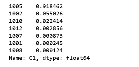
C1 value = 1005 has the most data, almost 92% of all the data we are using. Let’s see whether we can find value of C1 indicates something about CTR.

C1_values = train.C1.unique()
C1_values.sort()
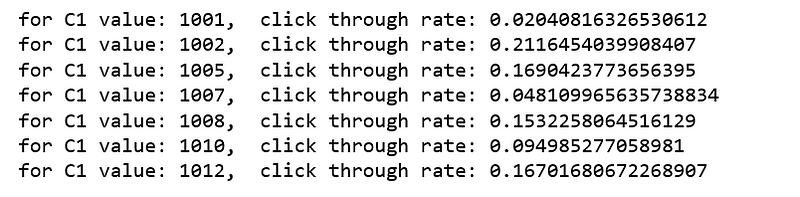
ctr_avg_list=[]
for i in C1_values:
    ctr_avg=train.loc[np.where((train.C1 == i))].click.mean()
    ctr_avg_list.append(ctr_avg)
    print("for C1 value: {},  click through rate: {}".format(i,ctr_avg))

Figure 13

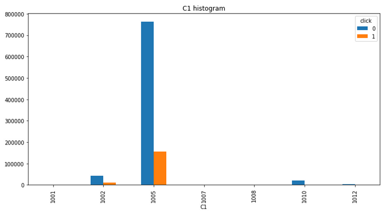
train.groupby(['C1', 'click']).size().unstack().plot(kind='bar', figsize=(12,6), title='C1 histogram');

Figure 14

df_c1 = train[['C1','click']].groupby(['C1']).count().reset_index()
df_c1 = df_c1.rename(columns={'click': 'impressions'})
df_c1['clicks'] = df_click[['C1','click']].groupby(['C1']).count().reset_index()['click']
df_c1['CTR'] = df_c1['clicks']/df_c1['impressions']*100

plt.figure(figsize=(12,6))
sns.barplot(y='CTR', x='C1', data=df_c1)
plt.title('CTR by C1');

Figure 15

The important C1 values and CTR pairs are:

C1=1005: 92% of the data and 0.17 CTR

C1=1002: 5.5% of the data and 0.21 CTR

C1=1010: 2.2% of the data and 0.095 CTR

C1 = 1002 has a much higher than average CTR, and C1=1010 has a much lower than average CTR, it seems these two C1 values are important for predicting CTR.

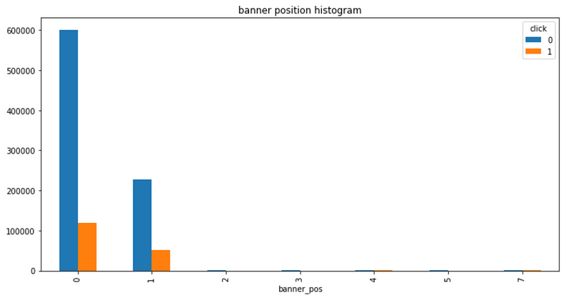
Banner position

I have heard that there are many factors that affect the performance of your banner ads, but the most influential one is the banner position. Let’s see whether it is true.

print(train.banner_pos.value_counts()/len(train))

Figure 16

banner_pos = train.banner_pos.unique()
banner_pos.sort()
ctr_avg_list=[]
for i in banner_pos:
    ctr_avg=train.loc[np.where((train.banner_pos == i))].click.mean()
    ctr_avg_list.append(ctr_avg)
    print("for banner position: {},  click through rate: {}".format(i,ctr_avg))

Figure 17

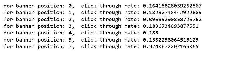
The important banner positions are:

position 0: 72% of the data and 0.16 CTR

position 1: 28% of the data and 0.18 CTR

train.groupby(['banner_pos', 'click']).size().unstack().plot(kind='bar', figsize=(12,6), title='banner position histogram');

Figure 18

df_banner = train[['banner_pos','click']].groupby(['banner_pos']).count().reset_index()
df_banner = df_banner.rename(columns={'click': 'impressions'})
df_banner['clicks'] = df_click[['banner_pos','click']].groupby(['banner_pos']).count().reset_index()['click']
df_banner['CTR'] = df_banner['clicks']/df_banner['impressions']*100
sort_banners = df_banner.sort_values(by='CTR',ascending=False)['banner_pos'].tolist()
plt.figure(figsize=(12,6))
sns.barplot(y='CTR', x='banner_pos', data=df_banner, order=sort_banners)
plt.title('CTR by banner position');

Figure 19

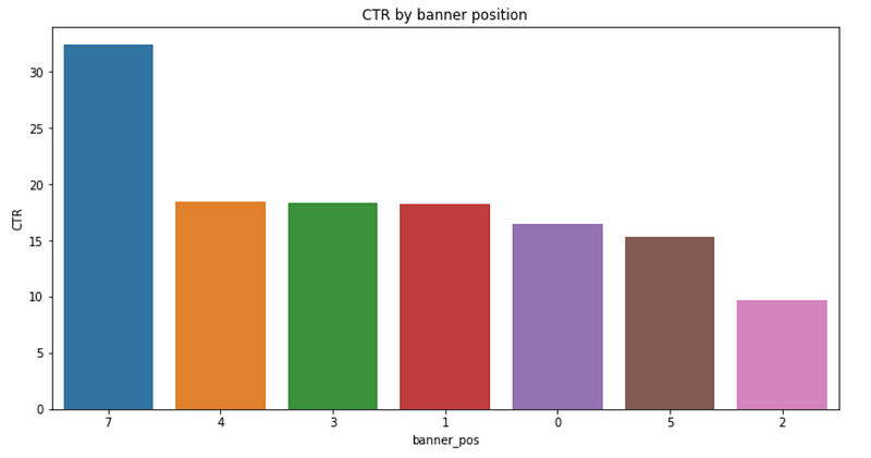
Although banner position 0 has the highest number of impressions and clicks, banner position 7 enjoys the highest CTR. Increasing the number of ads placed on banner position 7 seems to be a good idea.

Device type

print('The impressions by device types')
print((train.device_type.value_counts()/len(train)))

Figure 20

train[['device_type','click']].groupby(['device_type','click']).size().unstack().plot(kind='bar', title='device types');

Figure 21

Device type 1 gets the most impressions and clicks, and the other device types only get the minimum impressions and clicks. We may want to look in more details about device type 1.

df_click[df_click['device_type']==1].groupby(['hour_of_day', 'click']).size().unstack().plot(kind='bar', title="Clicks from device type 1 by hour of day", figsize=(12,6));

Figure 22

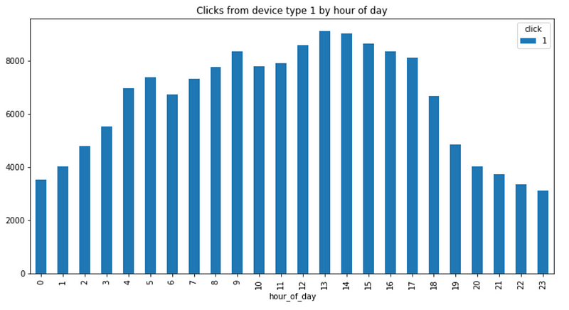
As expected, most clicks happened during the business hours from device type 1.

device_type_click = df_click.groupby('device_type').agg({'click':'sum'}).reset_index()
device_type_impression = train.groupby('device_type').agg({'click':'count'}).reset_index().rename(columns={'click': 'impressions'})
merged_device_type = pd.merge(left = device_type_click , right = device_type_impression, how = 'inner', on = 'device_type')
merged_device_type['CTR'] = merged_device_type['click'] / merged_device_type['impressions']*100

merged_device_type

Figure 23

The highest CTR comes from device type 0.

Using the same way, I explored all the other categorical features such as site features, app features and C14-C21 features. The way of exploring are similar, the details can be found on Github, I will not repeat here.

Building Models

Introducing Hash

A hash function is a function that maps a set of objects to a set of integers. When using a hash function, this mapping is performed which takes a key of arbitrary length as input and outputs an integer in a specific range.

Our reduced dataset still contains 1M samples and ~2M feature values. The purposes of the hashing is to minimize memory consumption by the features.

There is an excellent article on hashing tricks by Lucas Bernardi if you want to learn more.

Python has a built in function that performs a hash called hash(). For the objects in our data, the hash is not surprising.

def convert_obj_to_int(self):
    
    object_list_columns = self.columns
    object_list_dtypes = self.dtypes
    new_col_suffix = '_int'
    for index in range(0,len(object_list_columns)):
        if object_list_dtypes[index] == object :
            self[object_list_columns[index]+new_col_suffix] = self[object_list_columns[index]].map( lambda  x: hash(x))
            self.drop([object_list_columns[index]],inplace=True,axis=1)
    return self
train = convert_obj_to_int(train)

LightGBM Model

lightGBM_CTR

The final output after training:

Figure 24

Xgboost Model

Xgboost_CTR

It will train until eval-logloss hasn’t improved in 20 rounds. And the final output:

Figure 25

Jupyter notebook can be found on Github. Have a great weekend!